/ /

Graphs

You’ve learned about data structure that are built into Java, and you’ve learned about node-based data structures that use a Node class to model relationships between data.

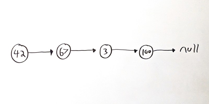
Specifically, you’ve seen linked lists, where each node contains a value and points to a single child node:

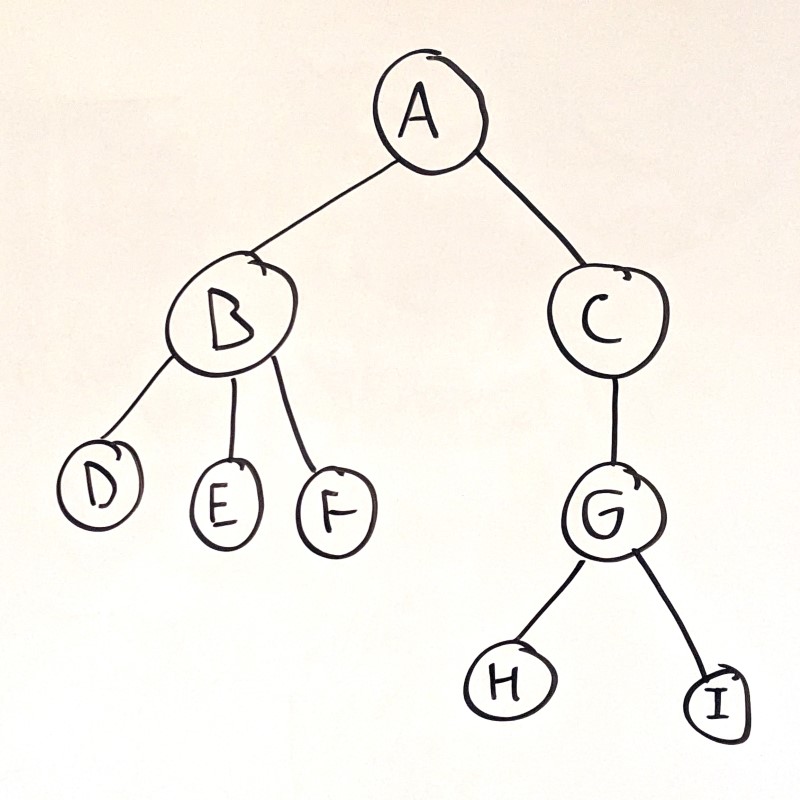
You’ve also seen trees, where each node can point to multiple child nodes:

Trees are good for modeling hierarchical data, or decision-making processes. In a tree, nodes have parent-child relationships.

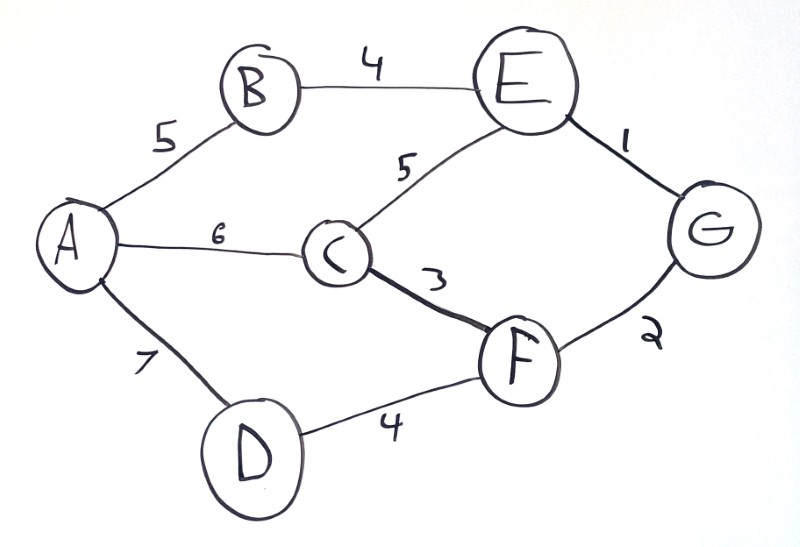
Graphs are another node-based data structure, but the relationships between nodes are not hierarchical:

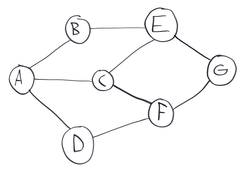
In this example, node A has three connected sibling nodes B, C, and D. Node B has two sibling nodes A and E. Node C has three sibling nodes A, E, and F, and so on.

Graphs can represent interconnected data, or physical spaces like streets or cities. It’s common to think about paths through graphs. In this example, there are several paths from A to G:

A -> B -> E -> G
A -> C -> E -> G
A -> C -> F -> G
A -> D -> F -> G

Connection Costs

In the above example, each node is connected to a set of other nodes. Each connection is yes-or-no: two nodes are either connected, or they’re not. Node A is connected to nodes B, C, and D, but it’s not connected directly to nodes E, F, or G.

A common enhancement to graphs is to include a cost (also called a weight) for each connection. You can think of this as the distance between two cities, or how much work it takes to get from one condition to the next.

Now each path has an associated cost:

A -> B -> E -> G costs 10
A -> C -> E -> G costs 12
A -> C -> F -> G costs 8
A -> D -> F -> G costs 13

The exact meaning behind costs depends on the problem. Costs are commonly associated with distance, but you can also think of it as how much work it takes to go from one node to another, or how desirable different paths are. For example, Google Maps sometimes highlights biking paths that might have a longer distance but will require less uphill pedaling.

You can also assign costs or weights to the nodes (also called vertexes) themselves.

Direction

The above examples assume that if two nodes are connected, they’re connected both ways. For example, if A is connected to B, then B is connected to A.

That means you can construct longer paths through the graph:

A -> B -> E -> C -> F -> G costs 19
A -> D -> F -> C -> E -> G costs 20

This is called an undirected or bidirectional graph.

Graphs can also be directed, which means connections are one-way. In visualizations, directed connections are often indicated by arrows:

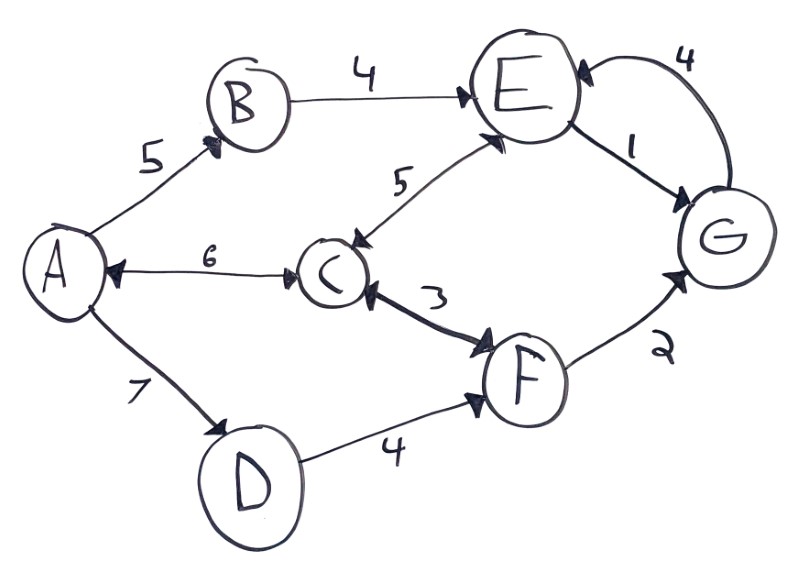
This example contains a few types of connections:

One-way (aka directed) connections, like from A to B
Two-way (aka undirected or bidirectional) connections, like between A and C
Connections with different costs depending on the direction, like how E to G costs 1 but G to E costs 4

Again, the meaning behind directionality in a graph depends on the problem you’re solving. You can think of them as one-way streets, or as unreversible decisions.

Cycles

A path inside a graph is considered a cycle if it starts and ends with the same node.

The above example contains a couple cycles:

A -> D -> F -> C -> A
C -> F -> G -> E -> C

Graphs containing cycles are called cyclic graphs, and graphs without cycles are acyclic.

Graphs that contain cycles require some extra care when traversing, to make sure you don’t get caught in an infinte loop. More on that below!

DAGs

Graphs can be directed or undirected, and cyclic or acyclic.

Graphs that are both directed (connections are one-way) and acyclic (no path loops back on itself) are so useful that they have their own nickname: DAG, which stands for directed acyclic graph.

DAGs are graphs that model a hierarchical relationship between data. Does that sound familiar? That’s because trees are DAGs, with one extra requirement of each node only having a single parent.

This is a DAG, but not a tree:

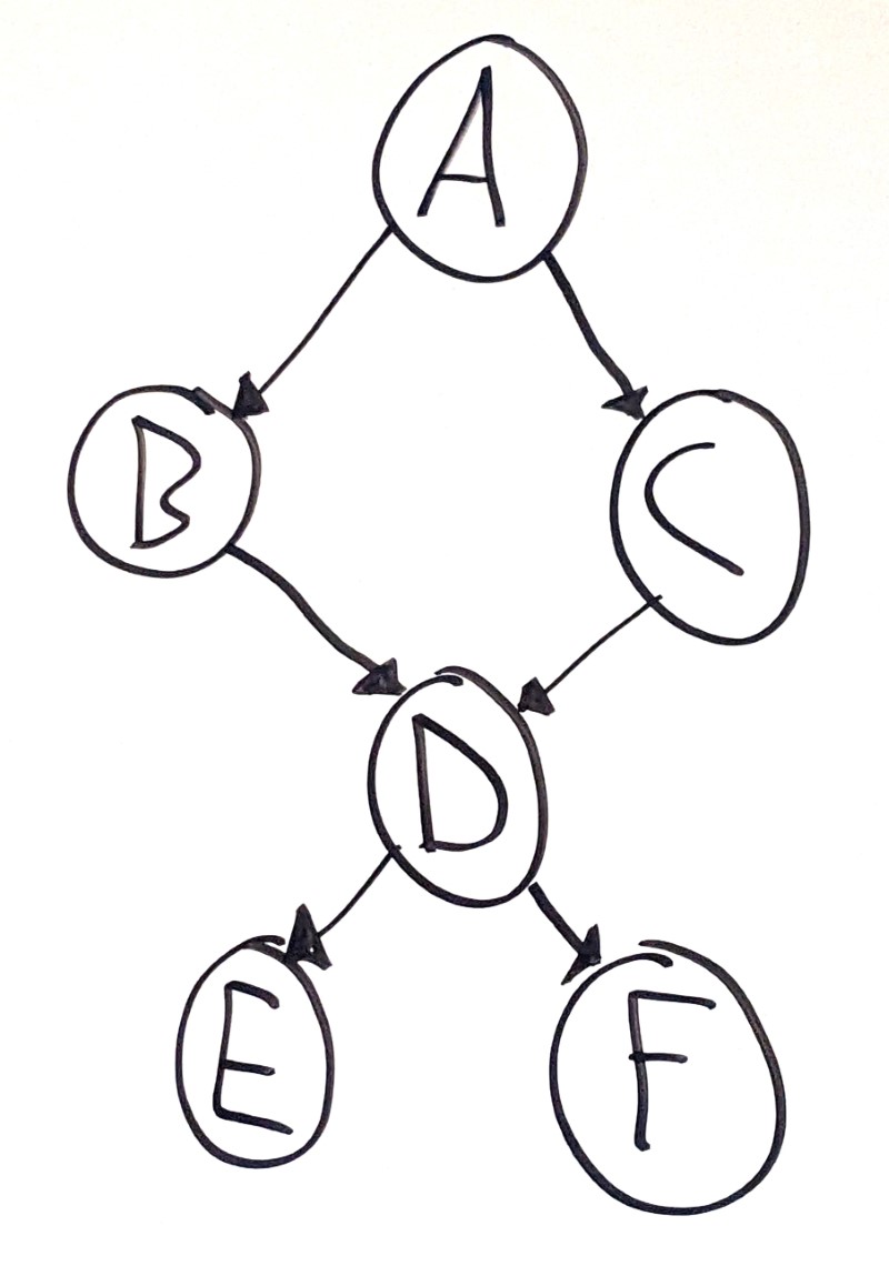
Node D has two parent nodes, which means it’s not a tree.

This is a tree, which is a specific type of DAG:

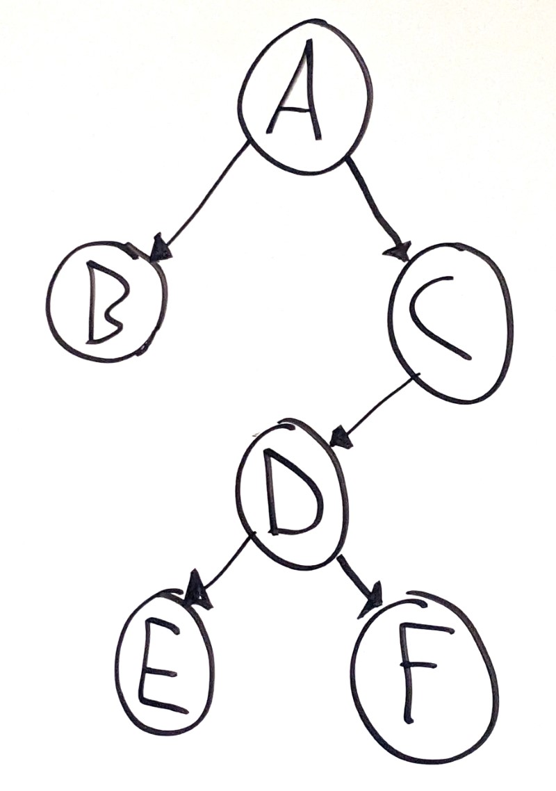
In other words, all trees are DAGs, but not all DAGs are trees.

To go a level deeper, linked lists are also DAGs. In fact, you can think of linked lists as a specific kind of tree where each node only has a single child!

Graph Representations

So far, we’ve focused on the concepts behind graphs, but we haven’t seen any code yet.

That’s because graphs can be represented in a ton of different ways.

Nodes

You could use a Node class:

class Node {
  Object value; // Could be int, String, etc.
  List<Node> neighbors;
}

You could also represent costs for each connection:

class Node {
  Object value; // Could be int, String, etc.
  Map<Node, Integer> connections; // Map of neighbors to costs.
}

List<Node> graph;

The Node class could work for a directed graph, but for a bidirectional graph you’d need to make sure every connection was reflected in both nodes.

Connection Lists

Alternatively, you could represent a graph by storing the connections as their own objects:

class Node {
  Object value;
}

class Connection {
  Node one;
  Node two;
}

List<Connection> graph;

With that approach, you can also represent directionality and costs by modifying the Connection class:

class Connection {
  Node source;
  Node destination;
  int cost;
}

Many Leetcode questions involving graphs provide the input in the form of a list of connections, usually 2D arrays where each inner array contains a source index, a destination index, and a cost.

int[][] graph = {
  {2, 3, 17}, // Connection from node 2 to node 3 with 17 cost
  {8, 1, 5},  // Connection from node 8 to node 1 with 5 cost
  {5, 6, 2}   // Connection from node 5 to node 6 with 2 cost
};

This example is directed and contains costs, but you’ll also encounter undirected graphs and graphs without costs in similar formats:

int[][] graph = {
  {2, 3}, // Connection between node 2 and node 3
  {8, 1}, // Connection between node 8 and node 1
  {5, 6}  // Connection between node 5 and node 6
};

Adjacency Matrixes

The above examples use Node or Connection classes to represent a graph. These object-based representations are handy if you think in terms of objects!

Another way to represent a graph is with a 2D array, where each row in the array represents the paths from a node to the other nodes in the graph. This is called an adjacency matrix.

In other words, you’d fill out the costs in a table like this:

		To Node
		A	B	C	D	E
From Node	A	x
	B		x
	C			x
	D				x
	E					x

Each row in the table represents a different node in the graph, and the cells in the row represent the cost of the connection from that node to another node. This table contains x values in the cells that connect a node to itself.

With this approach, your graph is a 2D array:

int[][] graph;

Each node in the graph is assigned an index. To check whether node 1 is connected to node 3, you can look it up in the array:

int costFromNodeOneToNodeThree = graph[1][3];

The exact values in the matrix depend on your problem and what type of graph you’re working with. You might use boolean values instead of costs. You might use 0 to represent a lack of a connection, or you might use infinity or null.

Adjacency Lists

Storing the connections as a list of node or index pairs makes it hard to look up whether a node is connected to another node. But storing the connections in a 2D array requires O(n ^ 2) space which takes up more space than most graphs need.

Instead, you can convert your connection list into an adjacency list, which is a list of connections for each node.

It looks like this:

int[][] graph = {
  {2, 3}, // Node 0 is connected to nodes 2 and 3.
  {0},    // Node 1 is connected to node 0.
  {0, 3}, // Node 2 is connected to nodes 0 and 3.
  {1}     // Node 3 is connected to node 1.
};

This example uses an array, but you could use a List<List<Integer>> or a Map<Integer, List<Integer>> as well.

You can also add a dimension for costs:

int[][] graph = {
  {{2, 7}, {3, 5}}, // Node 0 is connected to nodes 2 with cost 7 and 3 with cost 5.
  {{0, 6}},         // Node 1 is connected to node 0 with cost 6.
  {{0, 2}, {3, 9}}, // Node 2 is connected to nodes 0 with cost 2 and 3 with cost 9.
  {{1, 8}}          // Node 3 is connected to node 1 with cost 8.
};

Conceptually this is very similar to the Node object-based approach, but without going through objects. Both are valid, and you should use whichever approach makes the most sense to you.

Example Graph

As an example, take this graph:

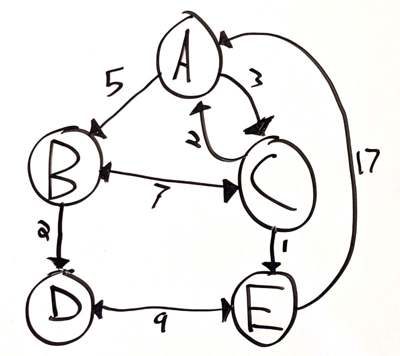
This is a directional graph, where each connection has a cost.

You could represent it using a Node class:

class Node {
  String name;
  Map<Node, Integer> connections = new HashMap<>();

  public Node(String name) {
    this.name = name;
  }

  public addConnection(Node neighbor, int cost){
    connections.put(neighbor, cost);
  }
}

Node a = new Node("A");
Node b = new Node("B");
Node c = new Node("C");
Node d = new Node("D");
Node e = new Node("E");

a.addConnection(b, 5);
a.addConnection(c, 3);
b.addConnection(c, 7);
b.addConnection(d, 2);
c.addConnection(a, 2);
c.addConnection(b, 7);
c.addConnection(e, 1);
d.addConnection(e, 9);
e.addConnection(a, 17);
e.addConnection(d, 9);

List<Node> graph = List.of(a, b, c, d, e);

Or you could use a Connection class:

class Connection {
  String fromNode; // Could also be a Node class.
  String toNode;
  int cost;

  public Connection(String fromNode, String toNode, int cost) {
    this.fromNode = fromNode;
    this.toNode = toNode;
    this.cost = cost;
  }
}

List<Connection> graph = new ArrayList<>();
graph.add(new Connection("A", "B", 5));
graph.add(new Connection("A", "C", 3));
graph.add(new Connection("B", "C", 7));
graph.add(new Connection("B", "D", 2));
graph.add(new Connection("C", "A", 2));
graph.add(new Connection("C", "B", 7));
graph.add(new Connection("C", "E", 1));
graph.add(new Connection("D", "E", 9));
graph.add(new Connection("E", "A", 17));
graph.add(new Connection("E", "D", 9));

Or you could use a table:

		To Node
		A	B	C	D	E
From Node	A	x	5	3	∞	∞
	B	∞	x	7	2	∞
	C	2	7	x	∞	1
	D	∞	∞	∞	x	9
	E	17	∞	∞	9	x

int[][] graph = {
  {0, 5, 3, 0, 0},
  {0, 0, 7, 2, 0},
  {2, 7, 0, 0, 1},
  {0, 0, 0, 0, 9},
  {17, 0, 0, 9, 0}
}

Or an adjacency list:

int[][][] graph = {
  // Node A is connected to Node 1 with 5 cost, and Node 2 with 3 cost.
  {{1, 5}, {2, 3}},
  // Node B is connected to Node C with 7 cost, and Node D with 3 cost.
  {{2, 7}, {3, 2}},
  // Node C is connected to Node A with 2 cost, Node B with 7 cost, and Node E with 1 cost.   
  {{0, 2}, {1, 7}, {4, 1}},
  // Node D is connected to Node E with 9 cost.
  {{4, 9}},
  // Node E is connected to Node A with 17 cost, and Node D with 9 cost.
  {{0, 17}, {3, 9}}
};

This adjacency list is a 3D array, where each row in the array represents a node, and each subarray represents a connection and cost. Again, you could use a List or a Map instead of an array.

The important thing to understand is that all of these representations reflect the same underlying graph!

Graph Algorithms

Graphs are used for many types of problem:

Pathfinding, like finding a route from one city to another
Dependency calculation, like checking prerequisites for college courses
Reasoning about connections, like tracking different groups

These problems generally require building answers by traversing the graph. Similar to trees, you can traverse a graph depth-first or breadth-first, recursively or iteratively.

Remember that depth-first search can be implemented recursively or with a stack, and breadth-first search can be implemented using a queue. One catch is that if you’re working with a graph that contains cycles, you also need to keep track of the nodes you already visited to avoid infinite loops.

For example, say you wanted to write a function that checks whether a bidirectional graph contains a path from one node to another.

Depth-First Search with Adjacency Matrix

You could do that with an adjacency matrix:

public boolean containsPath(boolean[][] graph, boolean[] visited, int startNode, int endNode) {
  // ...
}

This function takes four arguments:

graph is an adjacency matrix. If graph[2][3] is true, that means node 2 is connected to node 3.
visited is an array containing true for the node indexes that have already been visited. The first time this function is called, visited is filled with false values.
startNode is the index of the starting node.
endNode is the index of the ending node.

To implement depth-first search, you could call this function recursively to traverse the graph:

boolean containsPath(boolean[][] graph, boolean[] visited, int source, int destination) {
  // Base case. If the source is the destination, the algorithm has found a path.
  if(source == destination) {
    return true;
  }

  // Base case. If the source was already visited, stop exploring in this direction.
  if(visited[source]) {
    return false;
  }

  // Mark the source node as visited.
  visited[source] = true;

  // Check for connections from source to other nodes.
  for(int i = 0; i < graph[source].length; i++) {
    // If source is connected to node i, try exploring in the direction of node i.
    if(graph[source][i] && containsPath(graph, visited, i, destination)) {
      return true;
    }
  }

  // Couldn't find any paths to destination.'
  return false;
}

This recursive function has two base cases: one if the source and destination are equal, and one if source has already been visited. Then the code marks the current source as visited, and recursively calls the function with every connected neighbor.

Try stepping through this code with a few example graphs!

Depth-First Search with Nodes

You can also do the same thing with an object-based graph:

class Node {
  int index;
  List<Node> neighbors;
}

boolean containsPath(List<Node> graph, Set<Node> visited, Node source, Node destination) {
  // ...
}

Now, instead of an adjacency matrix, the function takes these arguments:

graph is a list of Node instances. Each Node stores its own connections.
visited is a Set that contains the already-visited nodes.
source is the starting node.
destination is the destination node.

The rest of the code is pretty similar to the adjacency matrix function, except now instead of looping through each index in the table row, the code loops through the current node’s neighbors:

boolean containsPath(List<Node> graph, Set<Node> visited, Node source, Node destination) {
  // Base case. If the source is the destination, the algorithm has found a path.
  if(source == destination) {
    return true;
  }

  // Base case. If the source was already visited, stop exploring in this direction.
  if(visited.contains(source)) {
    return false;
  }

  // Mark the source node as visited.
  visited.add(source);

  // Explore each connection from the current node.
  for(Node neighbor : source.neighbors) {
    if(containsPath(graph, visited, neighbor, destination)) {
      return true;
    }
  }

  // Couldn't find any paths to destination.'
  return false;
}

Breadth-First Search

And here’s the same problem, using breadth-first search:

boolean containsPath(List<Node> graph, Node source, Node destination) {
  // Keep track of which nodes were visited already.
  Set<Node> visited = new HashSet<>();

  // Breadth-first search queue of nodes.
  Queue<Node> nodeQueue = new ArrayDeque();
  nodeQueue.add(source);

  while(!nodeQueue.isEmpty()) {
    Node currentNode = nodeQueue.remove();

    // If the current node is the destination, the algorithm found a path.
    if(currentNode == destination) {
      return true;
    }

    // If the current node was already visited, skip it.
    if(visited.contains(currentNode)){
      continue;
    }

    // Mark the current node as visited.
    visited.add(currentNode);

    // Explore the current node's neighbors.
    nodeQueue.addAll(currentNode.neighbors);
  }

  // Couldn't find any paths to destination.'
  return false;
}

Adjacency Lists

Instead of using a Node class, you could use an adjacency list:

boolean containsPath(List<List<Integer>> graph, Set<Integer> visited, int source, int destination) {
  // Base case. If the source is the destination, the algorithm has found a path.
  if(source == destination) {
    return true;
  }

  // Base case. If the source was already visited, stop exploring in this direction.
  if(visited.contains(source)) {
    return false;
  }

  // Mark the source node as visited.
  visited.add(source);

  // Explore each connection from the current node.
  for(int neighbor : graph.get(source)) {
    if(containsPath(graph, visited, neighbor, destination)) {
      return true;
    }
  }

  // Couldn't find any paths to destination.
  return false;
}

Again, this code is very similar to the Node object-based approach, but it stores the connections in an adjacency list instead of a list of neighboring nodes.

Converting Input Data

With graph problems, half of the battle is taking the input data and converting it into a more useable format, like an adjacency matrix or a set of Node instances.

For example, this example problem is on Leetcode as Find if Path Exists in Graph. The input of that function is an array of edges, where each edge connects two node indexes.

public boolean validPath(int n, int[][] edges, int source, int destination) {
  // ...
}

By itself, that representation isn’t very useful. So the trick to the problem is converting the input into a more useful format.

This example builds an adjacency matrix and then calls the recursive function from above:

public boolean validPath(int n, int[][] edges, int source, int destination) {
  // Build an adjacency matrix.
  boolean[][] graph = new boolean[n][n];
  for(int[] edge : edges){
    graph[edge[0]][edge[1]] = true;
    graph[edge[1]][edge[0]] = true;
  }

  // Call the recursive containsPath function.
  return containsPath(graph, new boolean[n], source, destination);        
}

This example builds a List of Node instances and then calls the depth-first search or breadth-first search function from before:

class Node {
  int index;
  List<Node> neighbors = new ArrayList<>();

  public Node(int index) {
    this.index = index;
  }

  public void addNeighbor(Node neighbor){
    neighbors.add(neighbor);
  }
}

public boolean validPath(int n, int[][] edges, int source, int destination) {

  // Build a graph from Node instances.
  List<Node> graph = new ArrayList<>();
  for(int i = 0; i < n; i++) {
    graph.add(new Node(i));
  }

  for(int[] edge : edges){
    graph.get(edge[0]).addNeighbor(graph.get(edge[1]));
    graph.get(edge[1]).addNeighbor(graph.get(edge[0]));
  }

  // Call the recursive containsPath function.
  return containsPath(graph, new HashSet<>(), graph.get(source), graph.get(destination));
}

Finally, this example builds an adjacency list before calling the containsPath() function from above:

public boolean validPath(int n, int[][] edges, int source, int destination) {

  // Build an adjacency list.
  List<List<Integer>> graph = new ArrayList<>();
  for(int i = 0; i < n; i++) {
    graph.add(new ArrayList<>());
  }

  for(int[] edge : edges){
    graph.get(edge[0]).add(edge[1]);
    graph.get(edge[1]).add(edge[0]);
  }

  // Call the recursive containsPath function.
  return containsPath(graph, new HashSet<>(), source, destination);
}

In an interview environment, if having the graph in a particular format would make your life easier, ask your interviewer if the input can be in that format to start with. The worst case scenario is that they say no, but the best case scenario is that the problem becomes a lot easier to solve!

Learn More

Representing Graphs - Khan Academy

Practice Problems

Trees

Matrices